‘Welcome to Excel Avon
XLOOKUP Formula in Excel
XLOOKUP can work with vertical and horizontal data. The XLOOKUP function is a modern and flexible replacement for older functions such as LOOKUP, HLOOKUP, and VLOOKUP. Use the XLOOKUP function to find things in a row by row. For example, search bikes by bike price. With XLOOKUP, you can look in one column for the search term and return results from the same row in another column.
Formula
=XLOOKUP (lookup , lookup_array, return_array, [not_found], [match_mode], [search_mode])
Arguments
lookup – The value to search for.
lookup_array – The array or range in which lookup_range is to be searched
return_array – The array or range to return
not_found – [optional] the value to return in case the lookup value is not found. In case you don’t specify this argument, a #N/A error would be returned
match_mode – [optional] -1 = exact match or next smallest, 1 = exact match or next larger, 2 = wildcard match, 0 = exact match (default).
search_mode –search_mode – [optional] 1 = search from first (default), -1 = search from last, 2 = binary search ascending, -2 = binary search descending.
XLOOKUP Formula Examples
Download used excel file from here>>
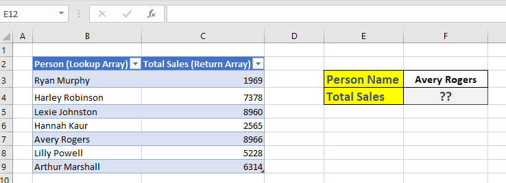
Example 1 : Exact match
These examples will help you better understand how XLOOKUP works, how it’s different from VLOOKUP and INDEX/MATCH. By the way, the Exact formula is a default, so as you can see there are two columns in the example, in which the data of the person and their cell is.
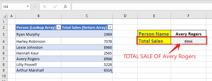
Suppose we know the total sales of a person (Avery Rogers),
then we will use the formula,
=XLOOKUP(F3,Table1[Person (Lookup Array)],Table1[Total Sales (Return Array)])
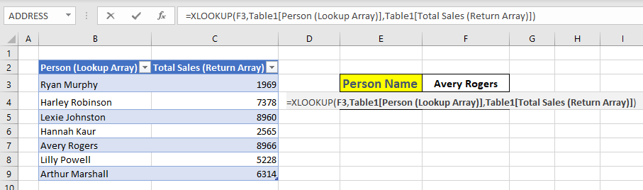
Where ‘F3’ is lookup, ‘B3:B9’ Is lookup_array and ‘C3:C9’ Is return_array. After Applying formula We will press enter and get the total sales of Avery Rogers.
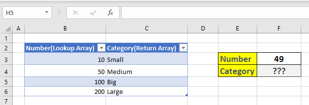
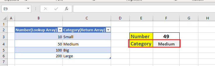
Example 2 : Approximate match with XLOOKUP formula
In this example in 2 columns we are given numbers and category. Many times it happens that we don’t have exact match, then we assume approximate and the formula returns the approximate value.
then we will use the XLOOKUP formula,
=XLOOKUP(F3,Table2[Number(Lookup Array)],Table2[Category(Return Array)],,1)
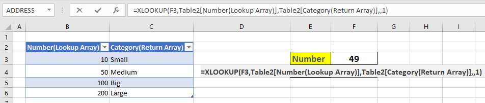
Where ‘F3’ is lookup, ‘B3:B6’ Is lookup_array and ‘C3:C6’ Is return_array. After Applying formula We will press enter and get the approximate category of 49.
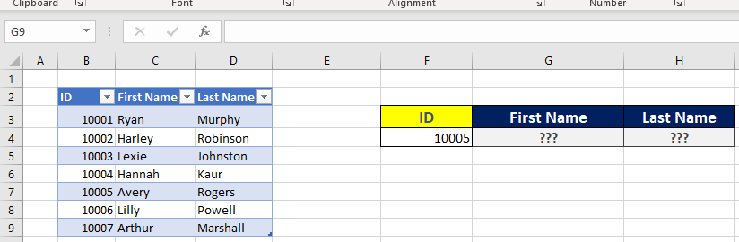
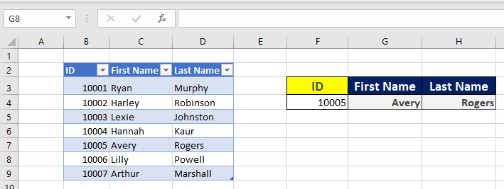
Example 3 : Return Multiple Values with XLOOKUP formula
We use Return Multiple Value Match when the return value is more than one. For example, we have made three columns and in which ID, first name and last name are given and based on id no we have to find the return value.
You can see example below.
then we will use the formula,
=XLOOKUP(F4,Table3[ID],Table3[[First Name]:[Last Name]])
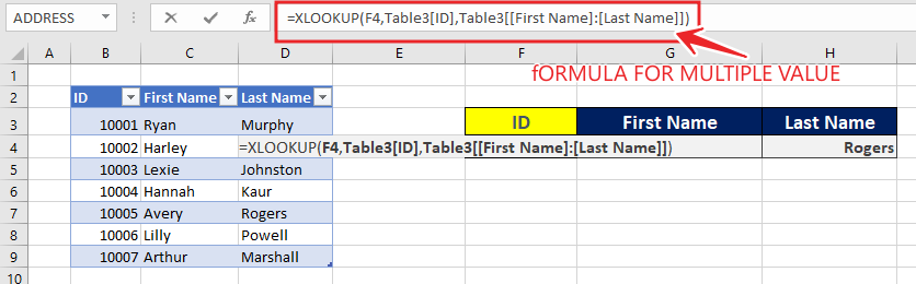
Where ‘F4’ is lookup, ‘B3:B9’ Is lookup_array and ‘C3:D9’ Is return_array. After Applying formula We will press enter and get the return value of ID 10005.
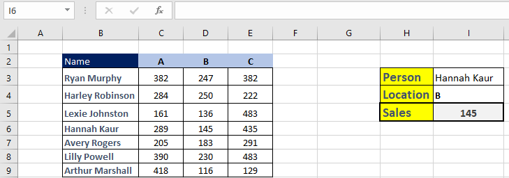
Example 4 : two-way lookup with XLOOKUP formula
2 way lookup is sometimes use when we need to lookup a value from table according to row title and column title. As can be seen in the 2 way lookup example some names are given in column B and some sale reports are given in column A, B and C then we have to find the sale report of Hannah Kaur’s location B like we have given two lookups so we have to use the lookup formula twice.
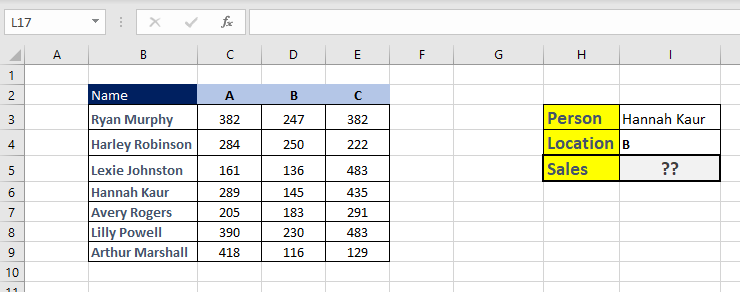
then we will use the XLOOKUP formula 2 times,
=XLOOKUP(I3,B3:B9,XLOOKUP(I4,C2:E2,C3:E9))
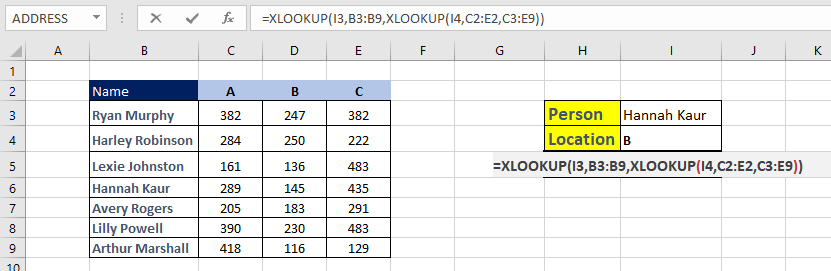
Where ‘I3’ & I4 is lookup, ‘B3:B9’ Is lookup_array and ‘C3:C9’ Is return_array. After Applying formula We will press enter and get the total sales of Hannah Kaur’s location B.
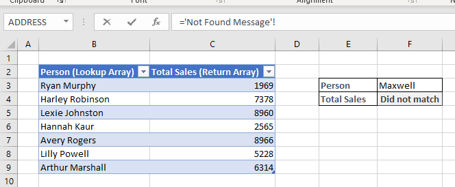
Example 5 : not found message with XLOOKUP formula
When the lookup array is not available, it returns the #N/A error. But In the given example some person has name(Lookup array) and their cells(return array) then we find cells from such lookup which is neither in lookup array nor in return array in this condition we will use ‘did not match’
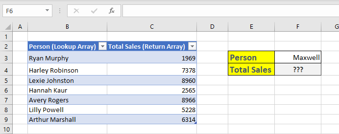
then we will use the formula,
=XLOOKUP(F3,Table15[Person (Lookup Array)],Table15[Total Sales (Return Array)],"Did not match")
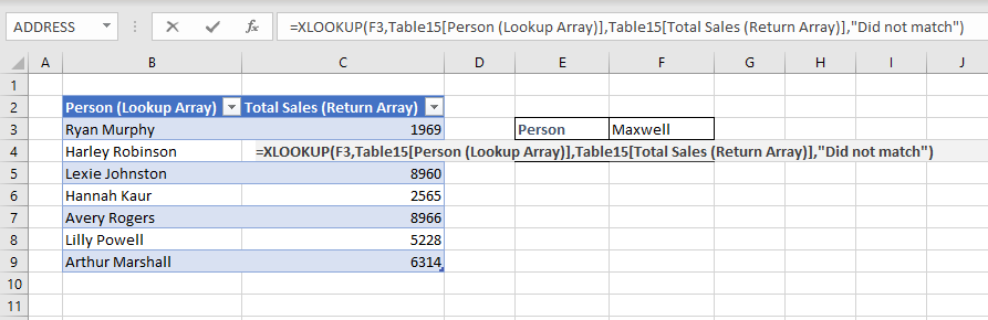
Where ‘F3’ is lookup, ‘B3:B9’ Is lookup_array and ‘C3:C9’ Is return_array. After Applying formula We will press enter and get the ‘did not match’.
Download used excel file from here>>
So I hope you have understood this formula and for more information you can follow us on Twitter, Instagram, LinkedIn and YouTube as well.
You can also see well explained video here
You can also read also similar formulas:
1. VLOOKUP Formula
")
")
